From rolling dice to differential equations: a discussion of four generating function problems
In this video blog post, I want to discuss the
four exercises that 3blue1brown left at the end of his latest video, plus some
additional background and context from the point of view of someone who works
with generating functions a lot.
Note: This article is, in a sense, the written counterpart to the manimated video I have produced for my YouTube channel. Feel free to check it out and leave a like in case you enjoyed it or found it helpful! :-)
At the end of 3blue1brown’s recent video on an innocent looking enumeration problem (which I highly recommend watching), he left four exercise problems. I do a lot with generating functions in my mathematical life, so I thought it would be a fun idea to discuss these four problems from my point of view – and I’ll also throw in some bonus material on top.
Before we jump into the problems, let me recommend some more literature: aside from Herbert Wilf’s Generatingfunctionology which Grant recommended in his video, I would also like to add to add Concrete Mathematics by Graham, Knuth, and Patashnik because I really like both the way how the book is written in general, as well as their approach of introducing generating functions in particular. And if you would like to see how the theory around generating functions can be developed further in a more analytical direction, I also want to recommend my favourite advanced book on that topic; the “purple bible”: Analytic Combinatorics by Flajolet and Sedgewick. If there is interest – let me know in the YouTube comments below my video! – I’ll talk a bit more about the very powerful, systematic approach to counting with generating functions described there in a future video.
Now, with that out of the way, let us discuss the four problems.
Problem 1: The Generating Function and the Expected Value
Problem statement: Take the derivative of both sides of \[ \frac{1}{1-x} = \sum_{n\geq 0} x^n. \] How can you use this to compute the expected number of times you have to roll a fair six-sided die before seeing the number 1?
Solution: The instructions from the first part of the problem are a bit clearer if we take a look at the second part of the problem, the one about the expected value, first: to determine the expected number of times we have to roll the die until we roll 1, we need to think about probabilities: We have a probability of $1/6$ to roll 1 with our first throw, in which case we had to wait for 0 throws before. Otherwise we rolled a non-1 (which happened with a probability of $5/6$) and now have to roll the die again. With a probability of $1/6$ we roll the 1 in our second attempt (which means we had to wait for 1 throw before), and with a probability of $5/6$ we – again – fail to get 1.
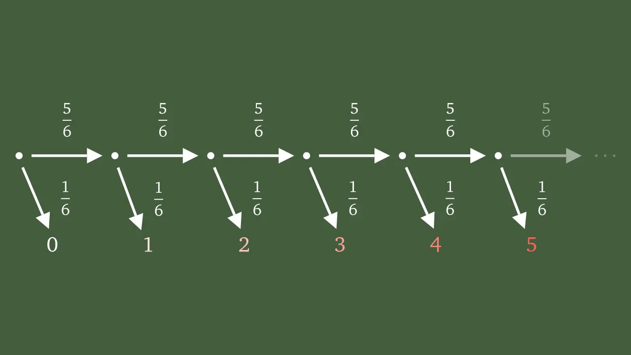
With the help of this diagram it is also not too hard to see that in general, the probability that we have to wait $n$ times before rolling 1 for the first time is $(5/6)^n \cdot (1/6)$.
To find the expected number of throws we have to wait for from there, we sum over all possible events (0 rolls before; 1 roll before; 2 rolls before, …) and multiply the number of times we had to wait with the corresponding probability. The sum we want to evaluate therefore is
\[ \begin{aligned} \mathbb{E} &= 0\cdot \frac{1}{6} + 1\cdot \frac{5}{6} \cdot \frac{1}{6} + 2 \cdot \bigg(\frac{5}{6}\bigg)^2 \frac{1}{6} + \cdots \\ & = \sum_{n\geq 0} n \cdot \bigg(\frac{5}{6}\bigg)^n \cdot \frac{1}{6}\\ & = \frac{1}{6} \sum_{n\geq 0} n \cdot \bigg(\frac{5}{6}\bigg)^n. \end{aligned} \]
This is as far as we can get at this point; let us now turn to the more “mechanical” part of the problem (taking derivatives) and then we will see how to combine the two parts.
Let me add some bonus content though: the sum on the right is a so-called geometric series, and from an analytic point of view it holds for all real (or complex) $x$ with absolute value less than 1. The identity can be derived directly, let us take a look: let $S_n = 1 + x + x^2 + \cdots + x^n$ denote the geometric sum of the terms from $1$ to $x^n$. Simply multiplying both sides with $x$ yields \[ x S_n = x + x^2 + x^3 + \cdots + x^{n+1}, \] a sum which shares almost all of its summands with the original $S_n$. And so, if we subtract $x S_n$ from $S_n$, we find \[ \begin{aligned} S_n - x S_n &= (1 + x + x^2 + \cdots + x^n) - (x + x^2 + \cdots + x^{n+1}) \\ &= 1 - x^{n + 1} \end{aligned} \] If we factor out $S_n$ on the left-hand side, we are left with $S_n (1 - x) = 1 - x^{n+1}$, or, as long as $x\neq 1$, \[ S_n = \frac{1 - x^{n+1}}{1 - x}. \] If we consider what happens when $n$ grows large (tends to infinity), then as long as $|x| < 1$, the term $x^{n+1}$ will tend to $0$. Everything else on the right-hand side does not depend on $n$, and such we have proved the identity for the geometric series, \[ 1 + x + x^2 + x^3 + \cdots = \frac{1}{1 - x}. \] A technical thing to note: given that we are differentiating an identity; in particular, something that holds in an entire neighborhood of $x = 0$ and not just for one particular value of $x$, we are allowed to take the derivative on both sides and we will obtain a valid equation again.
Differentiating the left-hand side gives (using the chain rule and the power rule): \[ \frac{\partial\,}{\partial x} \frac{1}{1 - x} = \frac{\partial\,}{\partial x} (1 - x)^{-1} = (-1)\cdot (1 - x)^{-2} \cdot (-1) = \frac{1}{(1 - x)^2}, \] and differentiating the right-hand side yields (by moving the derivative inside of the sum and then applying the power rule) \[ \frac{\partial\,}{\partial x} \sum_{n\geq 0} x^n = \sum_{n\geq 0} \frac{\partial\,}{\partial x} x^n = \sum_{n\geq 0} n x^{n-1}. \] Combining the two sides then gives us the useful identity \[ \frac{1}{(1 - x)^2} = \sum_{n\geq 0} n x^{n - 1}, \] which looks (unsurprisingly) familiar: if we multiply both sides with $x$ we arrive at \[ \frac{x}{(1 - x)^2} = \sum_{n\geq 0} n x^n, \] which helps us to evaluate the sum for the expected value $\mathbb{E}$ that we derived above: setting $x = 5/6$ gives, when reading from right to left, \[ \sum_{n\geq 0} n \cdot \bigg(\frac{5}{6}\bigg)^n = \frac{5/6}{(1 - 5/6)^2} = 30, \] and therefore we find that there are \[ \mathbb{E} = \frac{1}{6} \cdot 30 = 5 \] expected throws before we roll a 1 with a fair die.
Final note before we move on: the probability distribution that the number of throws before we hit 1 follows is the so-called geometric distribution (named like that because its probabilities form a geometric sequence).
Problem 2: A binomial sum
Problem statement: Compute the sum \[ \sum_{k=0}^n \binom{n}{k} 2^k. \]
Solution: This is a problem that I personally like a lot, and I will share some bonus material about it after discussing the solution. To solve this with the generating function approach, we make use of the binomial theorem, which states that for any non-negative integer $n$ and numbers $a$ and $b$ we have \[ (a + b)^n = \sum_{k=0}^{n} \binom{n}{k} a^k b^{n - k}. \] Observe that if we set $a = x$, and $b = 1$, that we find \[ (x + 1)^n = \sum_{k=0}^{n} \binom{n}{k} x^k. \] The right-hand side here already resembles the sum from the problem statement a lot, all that remains to do is to set $x = 2$ and the equation reads, from right to left, \[ \sum_{k=0}^{n} \binom{n}{k} 2^k = (2 + 1)^n = 3^n. \]
Bonus material: an alternative explanation
Identities like these are usually also an invitation to think about a more direct, combinatorial explanation. And it is not too hard to find one here: both sides of the equation \[ \sum_{k=0}^n \binom{n}{k} 2^k = 3^n \] express the number of possible colourings of the numbers from $1$ to $n$ with three colors (say red, green, blue):
- To arrive at the right-hand side, we go through all of the numbers one by one and pick one of the three possible colors for each of them. There are $n$ numbers with $3$ choices each, and therefore there are $3^n$ possible choices.
- And to obtain the left-hand side we first decide that $k$ of the numbers should either be red or green, then we choose these $k$ numbers in one of the $\binom{n}{k}$ possible ways, and decide for each of them whether it is red or green ($2$ choices for each of the $k$ numbers, thus $2^k$ possible choices). The remaining $n-k$ numbers that were not chosen are colored blue. For some specific $k$ we thus find $\binom{n}{k} 2^k$ possible colourings, and in order to obtain all possible colourings we have to sum over all possible values of $k$, from $k=0$ to $k=n$.
The fact that these two strategies with their corresponding counts both yield all possible colourings of the numbers from $1$ to $n$ with three colors proves that the identity holds. (In combinatorics, this sort of argument is usually referred to as double counting.)
Problem 3: Fibonacci numbers and a differential equation
Problem statement: Let $f_n$ be the $n$-th Fibonacci number and consider the generating function \[ F(x) = \sum_{n\geq 0} f_n \frac{x^n}{n!}. \] Explain why the differential equation $F^{\prime\prime}(x) = F’(x) + F(x)$ is true. For bonus points, solve this equation and use it to find a closed-form expression for $f_n$.
Solution: To find an explanation for the differential equation, we first investigate what happens if we differentiate a generating function of this particular shape; this is completely independent of $f_n$ being a Fibonacci number.
A generating function with the particular shape of $F(x)$, i.e., with the $n$-th coefficient being normalized by $n!$, is called exponential generating function. This is because the exponential function, as you might know, has the series expansion \[ e^x = 1 + x + \frac{x^2}{2} + \frac{x^3}{6} + \cdots = \sum_{n\geq 0} 1\cdot \frac{x^n}{n!}, \] that is, $e^x$ is the exponential generating function of the constant 1-sequence.
For the derivative of $F(x)$, we find \[ \begin{aligned} F’(x) &= \frac{\partial\,}{\partial x} \sum_{n\geq 0} f_n \frac{x^n}{n!} \\ &= \sum_{n\geq 0} \frac{\partial\,}{\partial x} f_n \frac{x^n}{n!} \\ &= \sum_{n\geq 0} f_n \frac{n x^{n-1}}{n!} \\ &= \sum_{n\geq 1} f_n \frac{x^{n-1}}{(n-1)!} \\ &= \sum_{n\geq 0} f_{n+1} \frac{x^n}{n!}. \end{aligned} \] In other words, if $F(x)$ is the exponential generating function of the sequence $f_0, f_1, f_2, \dots$, then $F’(x)$ is the exponential generating function of the shifted sequence $f_1, f_2, f_3, \dots$ – and we can simply apply the same argument again to see that the second derivative then is the exponential generating function of $f_2, f_3, f_4, \dots$. This is one of the most useful properties of exponential generating functions.
Now, back to our concrete situation where $f_n$ is the $n$-th Fibonacci number. By using the corresponding Fibonacci recurrence, $f_{n+2} = f_{n+1} + f_{n}$, we obtain \[ \begin{aligned} F^{\prime\prime}(x) &= \sum_{n\geq 0} f_{n+2} \frac{x^n}{n!} = \sum_{n\geq 0} (f_{n+1} + f_{n}) \frac{x^n}{n!}\\ &= \sum_{n\geq 0} f_{n+1} \frac{x^n}{n!} + \sum_{n\geq 0} f_n \frac{x^n}{n!}\\ &= F’(x) + F(x), \end{aligned} \] the differential equation we were asked to explain!
In general, this is a problem for which generating functions are very useful for, recurrences for sequences can often be translated into functional equations of their corresponding generating functions; and with a bit of luck, these equations can be solved to then give explicit formulas for the elements in the sequence. A very neat trick!
We also want to get full points from Grant, so let us solve the differential equation: without going into too much detail why this works, we use the Ansatz $F(x) = e^{\lambda x}$ (which means that we assume that the solution has a certain shape – you could say that we are just making an educated guess and then see how far we can take it), where $\lambda$ is a constant. Plugging it into the differential equation and bringing everything to one side gives \[ \lambda^2 e^{\lambda x} - \lambda e^{\lambda x} - e^{\lambda x} = 0. \] Now, because $e^{\lambda x}$ is never zero we may conclude that if our Ansatz should work, the equation \[ \lambda^2 - \lambda - 1 = 0 \] has to hold – and indeed, we find that \[ \lambda_+ = \frac{1 + \sqrt{5}}{2}, \quad \lambda_- = \frac{1 - \sqrt{5}}{2} \] are solutions to the quadratic equation (and at this point we, obligatorily, have to point out that $\lambda_+$ is “coincidentally” $\varphi$, the golden ratio).
You can convince yourself that we actually just found some solutions to the differential equation, both $x\mapsto e^{\lambda_+ x}$ as well as $x\mapsto e^{\lambda_- x}$ satisfy $F^{\prime\prime}(x) = F’(x) + F(x)$ – and so does a linear combination of the two, $x\mapsto c_+ e^{\lambda_+ x} + c_- e^{\lambda_- x}$ for constants $c_-$ and $c_+$; plug the functions into the differential equation and you will see that it all works out.
However, we are not looking for any solution to the differential equation, we are looking for a fairly specific one: the solution should be the generating function for Fibonacci numbers, after all! To nail down the particular solution we are looking for, we have to use some information of the generating function – for example, that we want to have $F(0) = f_0 = 0$, the $0$-th Fibonacci number, and the derivative as the generating function of the shifted sequence should satisfy $F’(0) = f_1 = 1$.
Plugging these conditions into the general solution, \[ F(x) = c_+ e^{\lambda_+ x} + c_- e^{\lambda_- x} \] translates to the equations $c_+ + c_- = 0$, and $c_+ \lambda_+ + c_- \lambda_- = 1$. Plugging $c_- = - c_+$ (from the first equation) into the second one yields \[ 1 = c_+ \lambda_+ - c_+ \lambda_- = c_+ (\lambda_+ - \lambda_-), \] and a straightforward computation gives $\lambda_+ - \lambda_- = \sqrt{5}$ so that we arrive at $c_+ = 1/\sqrt{5}$ and $c_- = -1\sqrt{5}$.
Overall, this implies \[ F(x) = \frac{1}{\sqrt{5}} e^{\lambda_+ x} - \frac{1}{\sqrt{5}} e^{\lambda_- x}, \] and the explicit formula for $f_n$ can now be obtained by rewriting the exponential functions into their series representation, \[ \begin{aligned} F(x) &= \frac{1}{\sqrt{5}} \sum_{n\geq 0} \lambda_+^n \frac{x^n}{n!} - \frac{1}{\sqrt{5}} \sum_{n\geq 0} \lambda_-^n \frac{x^n}{n!} \\ &= \sum_{n\geq 0} \frac{1}{\sqrt{5}} (\lambda_+^n - \lambda_-^n) \frac{x^n}{n!}. \end{aligned} \] This proves Binet’s explicit formula for the $n$-th Fibonacci number: \[ f_n = \frac{1}{\sqrt{5}} \bigg(\bigg(\frac{1 + \sqrt{5}}{2}\bigg)^n - \bigg(\frac{1 - \sqrt{5}}{2}\bigg)^n\bigg). \]
Problem 4: A useful product
Problem statement: Suppose $f(x) = \sum_{n\geq 0} a_n x^n$. What do the coefficients of \[ \frac{f(x)}{1 - x} \] tell you?
Solution: This final problem is a bit shorter again, but invites us to prove a very useful sequence construction with many applications: for example, one can use this in the average case analysis of Quicksort (and if that has made you curious, let me know; I might discuss this in a future video … :-) ).
Here is how we can tackle this: \[ \begin{aligned} \frac{f(x)}{1 - x} &= \frac{1}{1-x} \sum_{\ell\geq 0} a_{\ell} x^{\ell} = \sum_{\ell\geq 0} a_{\ell} \frac{x^{\ell}}{1 - x}\\ &= \sum_{\ell\geq 0} a_{\ell} x^{\ell} (1 + x + x^2 + \cdots) \\ &= \sum_{\ell\geq 0} a_{\ell} (x^{\ell} + x^{\ell+1} + x^{\ell+2} + \cdots) \\ &= \sum_{\ell\geq 0} a_{\ell} \sum_{n\geq \ell} x^{n}. \end{aligned} \] The trick to make this expression nicer is to change the order of summation. The following image should help to visualize the situation:
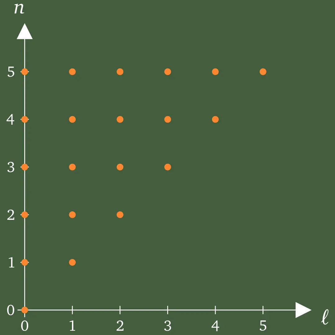
In the grid, every cell corresponds to one summand. In the original sum, we first iterate over the columns ($\ell\geq 0$), and then sum over all cells once we have passed a certain threshold ($n \geq \ell$). If we change the order of summation, we first iterate over the rows ($n \geq 0$), and then over all cells up to a certain column threshold ($0\leq \ell\leq n$).
Practically, this means that we rewrite \[ \sum_{\ell\geq 0} a_{\ell} \sum_{n\geq \ell} x^{n} = \sum_{n\geq 0} \bigg(\sum_{\ell = 0}^{n} a_{\ell} \bigg) x^{n}, \] or alternatively, in the expanded form, \[ a_0 (1 + x + x^2 + x^3 + \cdots) + a_1 (x + x^2 + x^3 + \cdots) + a_2 (x^2 + x^3 + \cdots) + a_3 (x^3 + \cdots) + \cdots \] becomes \[ a_0 + (a_0 + a_1)x + (a_0 + a_1 + a_2)x^2 + (a_0 + a_1 + a_2 + a_3)x^3 + \cdots. \] This representation allows us to read off the coefficients of $f(x)/(1-x)$: if $f(x)$ is the generating function with coefficient sequence $a_0, a_1, a_2, \dots$, then $f(x)/(1-x)$ has coefficient sequence \[ a_0, a_0 + a_1, a_0 + a_1 + a_2, a_0 + a_1 + a_2 + a_3, \dots, \] that is, partial sums of the original sequence.
And this concludes the discussion of the solutions of the four problems. Let me know in the YouTube comments: did you find this helpful? Are you curious about more generating function “magic”?
Thank you very much for watching reading, and see you in the
next video blog post!